Polygon Field Flagging

This example demonstrates end-to-end polygon-based flagging:

1. Build a regular block model.

2. Define a named PolygonField from Shapely geometry.

3. Visualise the polygon against block centroids in 2D.

4. Evaluate a boolean mask from centroid-in-polygon tests (XY only).

5. Encode the result as a categorical block-model attribute.

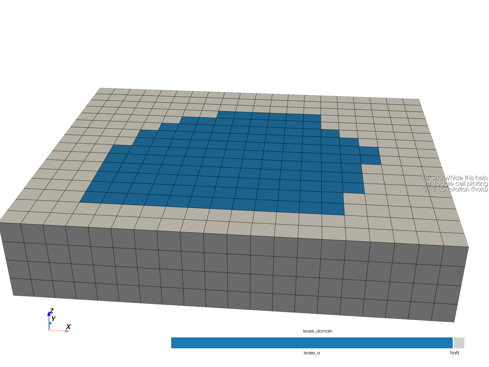
6. Plot the final 3D block model by that categorical flag.

import tempfile
from pathlib import Path

import geopandas as gpd
import matplotlib.pyplot as plt
import numpy as np
import pandas as pd
import pyvista as pv
from shapely.geometry import Polygon

from parq_blockmodel import ParquetBlockModel, PolygonField, RegularGeometry

Create a geometry-backed block model

We start from geometry only, then materialise a canonical .pbm.

temp_dir = Path(tempfile.gettempdir()) / "polygon_field_flagging_example"
temp_dir.mkdir(parents=True, exist_ok=True)
pbm_path = temp_dir / "polygon_field_flagging.pbm"

geometry = RegularGeometry(
    corner=(0.0, 0.0, 0.0),
    block_size=(1.0, 1.0, 1.0),
    shape=(20, 16, 4),
)

pbm = ParquetBlockModel.from_geometry(geometry=geometry, path=pbm_path)
blocks = pbm.read(index=None)

Persist and ingest a named polygon field (GeoParquet)

We write a simple named polygon table and then ingest by name. This demonstrates the persisted polygon interchange pattern.

lease_outline = Polygon(
    [
        (3.0, 2.0),
        (15.0, 2.5),
        (17.0, 8.0),
        (13.0, 13.5),
        (6.0, 12.0),
        (2.5, 7.0),
    ]
)
polygon_path = temp_dir / "lease_regions.parquet"
regions = gpd.GeoDataFrame(
    {"name": ["lease_a"], "geometry": [lease_outline]},
    crs="EPSG:4326",
)
regions.to_parquet(polygon_path)
polygon = PolygonField.from_geoparquet(polygon_path, name="lease_a")

print("Polygon name:", polygon.name)

Polygon name: lease_a

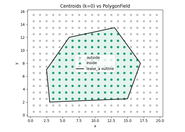
Visualise the polygon against centroid locations in 2D

Evaluation is strictly in world XY; Z is ignored.

mask = polygon.evaluate(pbm.geometry)
first_layer = blocks.loc[blocks["k"] == 0, ["block_id", "x", "y"]].copy()
first_layer["inside"] = mask[first_layer["block_id"].to_numpy(dtype=np.int64)]

fig, ax = plt.subplots(figsize=(7, 5))
ax.scatter(
    first_layer.loc[~first_layer["inside"], "x"],
    first_layer.loc[~first_layer["inside"], "y"],
    s=24,
    color="#bdbdbd",
    label="outside",
)
ax.scatter(
    first_layer.loc[first_layer["inside"], "x"],
    first_layer.loc[first_layer["inside"], "y"],
    s=28,
    color="#1b9e77",
    label="inside",
)

poly_x, poly_y = polygon.geometry.exterior.xy
ax.plot(poly_x, poly_y, color="#222222", linewidth=2.0, label=f"{polygon.name} outline")
ax.fill(poly_x, poly_y, color="#1b9e77", alpha=0.12)

ax.set_title("Centroids (k=0) vs PolygonField")
ax.set_xlabel("x")
ax.set_ylabel("y")
ax.set_aspect("equal", adjustable="box")
ax.legend(loc="best")
fig.tight_layout()
plt.show()

Encode the boolean mask as a categorical block-model attribute

We map True to the polygon name and False to missing (NA).

inside_label = polygon.name or "inside"

domain = np.full(len(blocks), pd.NA, dtype=object)
domain[mask[blocks["block_id"].to_numpy(dtype=np.int64)]] = inside_label
blocks["lease_domain"] = pd.Categorical(domain, categories=[inside_label], ordered=False)

pbm.write(blocks[["block_id", "lease_domain"]], merge=True)
print("lease_domain (NA-aware):")
print(pbm.read(columns=["lease_domain"], index=None)["lease_domain"].value_counts(dropna=False))

lease_domain (NA-aware):
lease_domain
NaN        776
lease_a    504
Name: count, dtype: int64

Plot the final 3D block model using the encoded categorical domain

plotter: pv.Plotter = pbm.plot(scalar="lease_domain", threshold=False, enable_picking=True, grid_type="image")
# Keep perspective, but bias the camera toward an XY-aligned oblique view so
# the 3D display is easier to relate to the 2D polygon map above.
b = plotter.bounds  # xmin, xmax, ymin, ymax, zmin, zmax
cx = 0.5 * (b[0] + b[1])
cy = 0.5 * (b[2] + b[3])
cz = 0.5 * (b[4] + b[5])
dx = b[1] - b[0]
dy = b[3] - b[2]
span_xy = max(dx, dy)
plotter.camera_position = [
    (cx + 0.15 * dx, cy - 2.0 * dy, cz + 0.9 * span_xy),  # camera position
    (cx, cy, cz),  # focal point
    (0.0, 0.0, 1.0),  # up-vector
]
plotter.show()