Regular Geometry

The underlying geometry (a.k.a. grid) is the foundation of a block model. Since parq-blockmodel is designed to work with regular geometries, this example demonstrates the underlying regular geometry by visualising it with PyVista.

import tempfile

import pandas as pd
from pathlib import Path

from seaborn import axes_style

from parq_blockmodel import ParquetBlockModel, RegularGeometry

Create Geometry

We RegularGeometry object (not a ParquetBlockModel). The geometry knows nothing about attributes, it only knows about the underlying geometry of the block model.

corner: tuple[float, float, float] = (0.0, 0.0, 0.0)
block_size: tuple[float, float, float] = (1.0, 1.0, 1.0)
shape: tuple[int, int, int] = (2, 2, 2)

geom: RegularGeometry = RegularGeometry(shape=shape,
                                        block_size=block_size,
                                        corner=corner
                                        )

geom

RegularGeometry: {'corner': (0.0, 0.0, 0.0), 'axis_angles': (0.0, 0.0, 0.0), 'block_size': (1.0, 1.0, 1.0), 'block_count': 8, 'shape': (2, 2, 2), 'is_regular': True, 'extents': ((0.0, 2.0), (0.0, 2.0), (0.0, 2.0)), 'bounding_box': ((0.0, 2.0), (0.0, 2.0))}

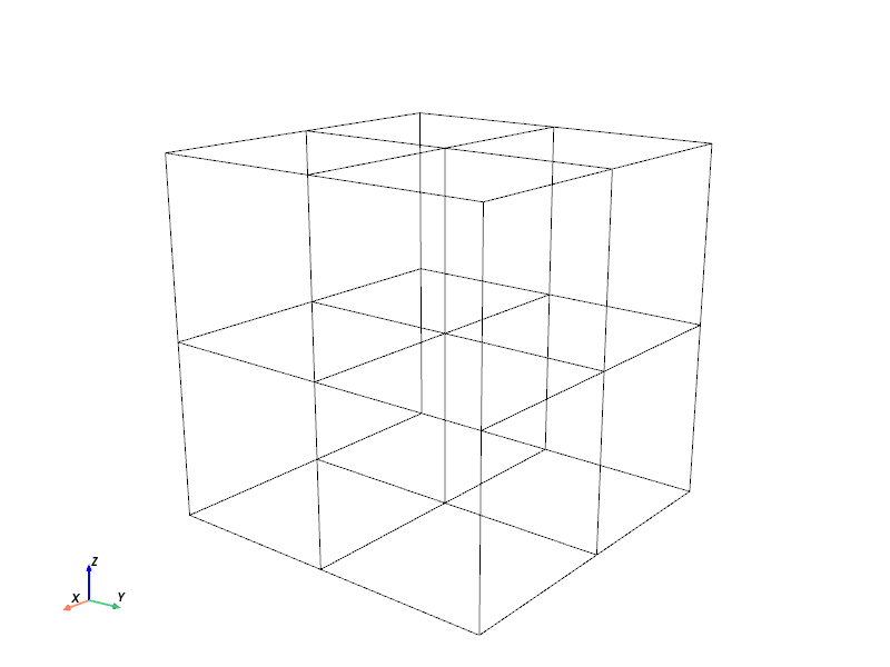
Visualise in 3D

Plot using PyVista. The geometry is a mesh, so we can use the plot method to visualise it.

import pyvista as pv

isometric_view = [
    (6, 5, 3),  # camera position
    (1, 1, 1),  # focal point (center of the grid)
    (0, 0, 1),  # view up direction
]

# Create a PyVista plotter
plotter = pv.Plotter()
edges = geom.to_pyvista().extract_all_edges()
plotter.add_mesh(edges, color="black", line_width=1)
plotter.show_axes()
plotter.camera_position = isometric_view
plotter.show(title="Regular Geometry", window_size=(800, 600))

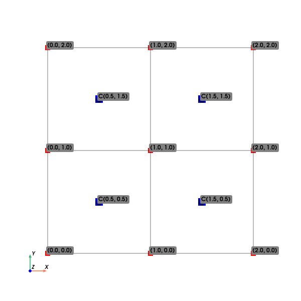
Visualise in 2D

In most cases a 2D visualisation is sufficient to understand the underlying geometry. We can use the to_pyvista method to get a PyVista mesh and then plot it in 2D.

grid = geom.to_pyvista()
# Slice at z=0.5 to intersect the first layer of cells
slice_2d = grid.slice(normal='z', origin=(0, 0, 0.5))
edges_2d = slice_2d.extract_all_edges()

points = edges_2d.points
labels = [f"({x:.1f}, {y:.1f})" for x, y, _ in points]

centroids_mesh = slice_2d.cell_centers()
centroids = centroids_mesh.points
labels_centroids_2d = [f"C({x:.1f}, {y:.1f})" for x, y, _ in centroids]

plotter = pv.Plotter()
plotter.add_mesh(edges_2d, color="black", show_edges=True)
plotter.add_point_labels(points, labels, font_size=12, point_color="red", point_size=10)
plotter.add_points(centroids, color="blue", point_size=15, render_points_as_spheres=True)
plotter.add_point_labels(centroids,
                         labels_centroids_2d,
                         font_size=12,
                         point_color="blue",
                         point_size=0,  # Hide label points
                         always_visible=True,
                         render_points_as_spheres=False)
plotter.show_axes()
plotter.view_xy()
plotter.show(title="2D Slice with Corner and Centroid Coordinates", window_size=(600, 600))