Load Block Model

Demonstrates loading a block model in parquet format into pyvista.

import logging
from pathlib import Path

import numpy as np
import pandas as pd
import pyvista as pv

from elphick.geomet import Sample
from elphick.geomet.block_model import BlockModel

logging.basicConfig(level=logging.DEBUG)

Load

block_model_filepath: Path = Path("block_model_copper.parquet")

# Load the parquet file into a DataFrame
df = pd.read_parquet(block_model_filepath)
print(df.shape)
df.head()

(1689600, 1)

			CU_pct
x	y	z
444705.0	492805.0	2335.0	0.002696
444715.0	492805.0	2335.0	0.002760
444725.0	492805.0	2335.0	0.002826
444735.0	492805.0	2335.0	0.002894
444745.0	492805.0	2335.0	0.002964

Create a BlockModel

The BlockModel class is a subclass of MassComposition and inherits all its attributes and methods. The block model plotted below is regular, that is, it has a record for every block in the model. Blocks are the same size and adjacent to each other. The block model is created from a DataFrame that has columns for the x, y, z coordinates and the copper percentage.

We need to assign a dry mass (DMT) to the block model to conform to the underlying MassComposition class.

bm: BlockModel = BlockModel(data=df.rename(columns={'CU_pct': 'Cu'}).assign(**{'DMT': 2000}),
                            name='block_model', moisture_in_scope=False)
bm._mass_data.head()
print(bm.is_irregular)
print(bm.common_block_size())

False
(np.float64(10.0), np.float64(10.0), np.float64(10.0))

bm.data.head()

			DMT	Cu
x	y	z
444705.0	492805.0	2335.0	2000	0.002696
444715.0	492805.0	2335.0	2000	0.002760
444725.0	492805.0	2335.0	2000	0.002826
444735.0	492805.0	2335.0	2000	0.002894
444745.0	492805.0	2335.0	2000	0.002964

Plot the block model

bm.plot('Cu').show(auto_close=False)

Filter the data

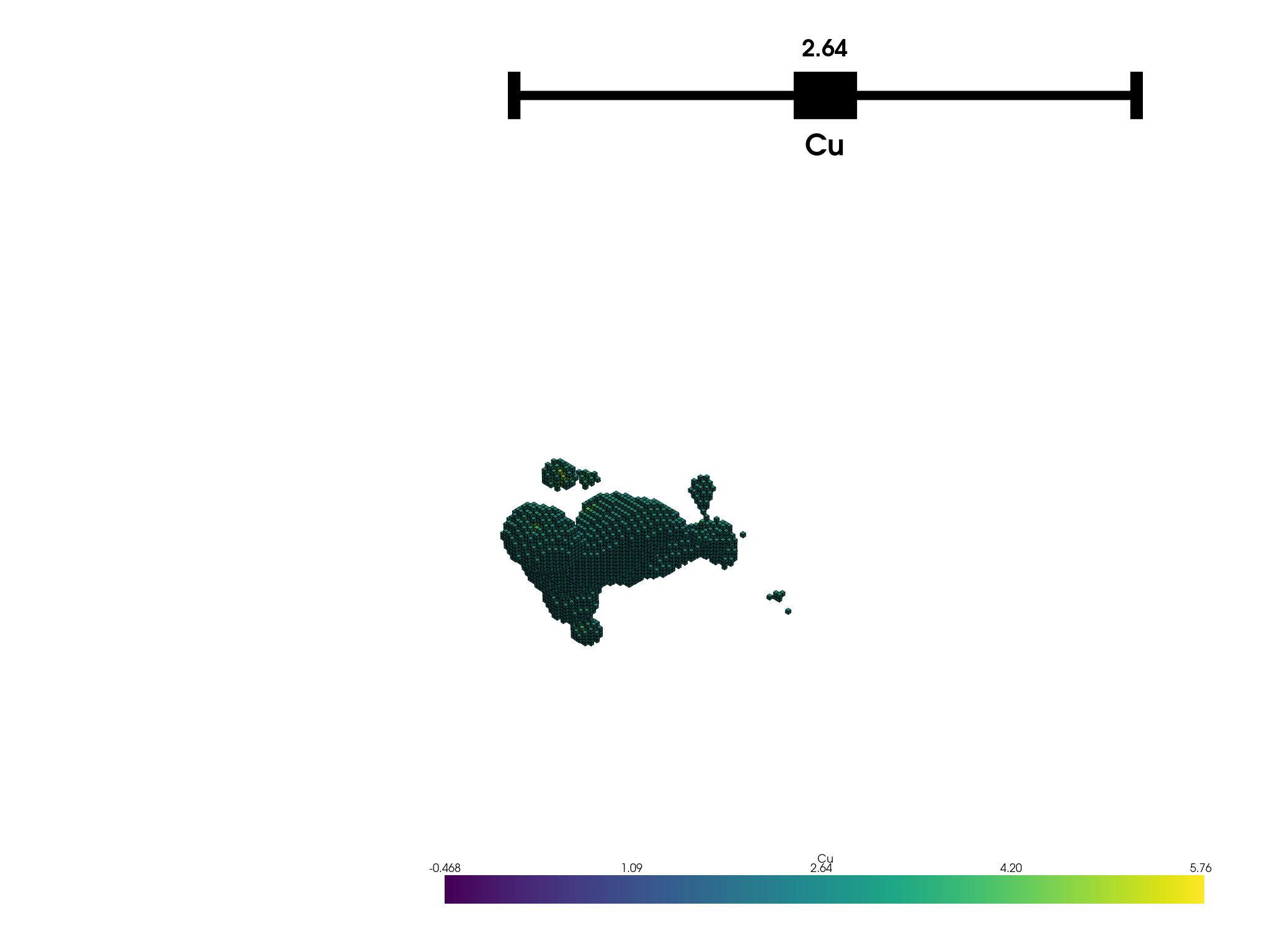
When a dataframe that represents a regular block model (a record for every block) is filtered, the resulting block model cannot be regular anymore. This is because the filtering operation may remove blocks that are adjacent to each other, resulting in a block model that is irregular. This example demonstrates this behavior. The plot below is generated from a filtered block model that was originally regular.

df_filtered = df.query('CU_pct > 0.132').copy()
bm2: BlockModel = BlockModel(data=df_filtered.rename(columns={'CU_pct': 'Cu'}).assign(**{'DMT': 2000}),
                             name='block_model', moisture_in_scope=False)
bm2._mass_data.shape

(766492, 2)

bm2.plot('Cu').show(auto_close=False)