Create Block Model

We leverage the omfvista block model example. We load the model and convert to a parquet.

Later, we may use this model along with a correlation matrix for an iron ore dataset to create a pseudo-realistic iron ore block model for testing.

We can also up-sample the grid to create larger datasets for testing.

# REF: https://opengeovis.github.io/omfvista/examples/load-project.html#sphx-glr-examples-load-project-py

import omfvista
import pooch
import pyvista as pv
import pandas as pd
from omf import VolumeElement
from ydata_profiling import ProfileReport

Load

# Base URL and relative path
base_url = "https://github.com/OpenGeoVis/omfvista/raw/master/assets/"
relative_path = "test_file.omf"

# Create a Pooch object
p = pooch.create(
    path=pooch.os_cache("geometallurgy"),
    base_url=base_url,
    registry={relative_path: None}
)

# Use fetch method to download the file
file_path = p.fetch(relative_path)

# Now you can load the file using omfvista
project = omfvista.load_project(file_path)
print(project)

MultiBlock (0x7f90cc7a5960)
  N Blocks    9
  X Bounds    443941.105, 447059.611
  Y Bounds    491941.536, 495059.859
  Z Bounds    2330.000, 3555.942

project.plot()

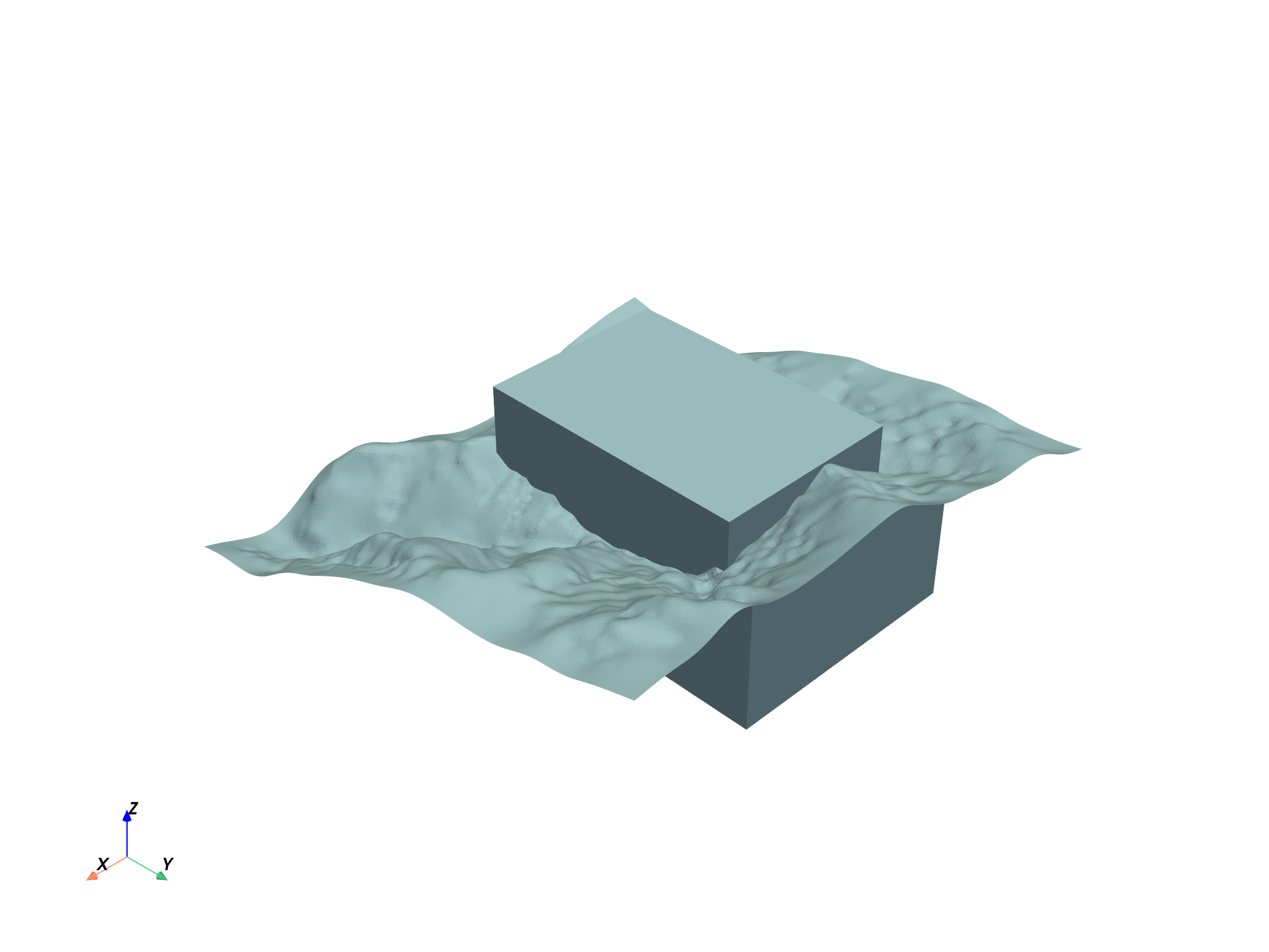
vol = project["Block Model"]
assay = project["wolfpass_WP_assay"]
topo = project["Topography"]
dacite = project["Dacite"]

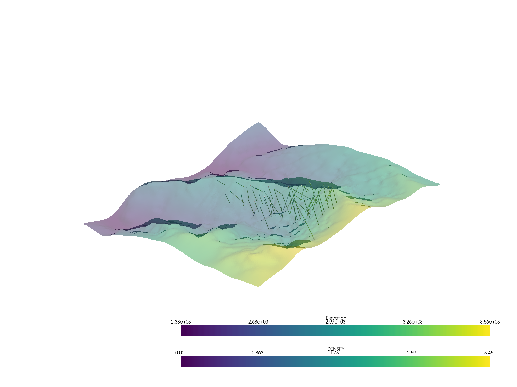
assay.set_active_scalars("DENSITY")

p = pv.Plotter()
p.add_mesh(assay.tube(radius=3))
p.add_mesh(topo, opacity=0.5)
p.show()

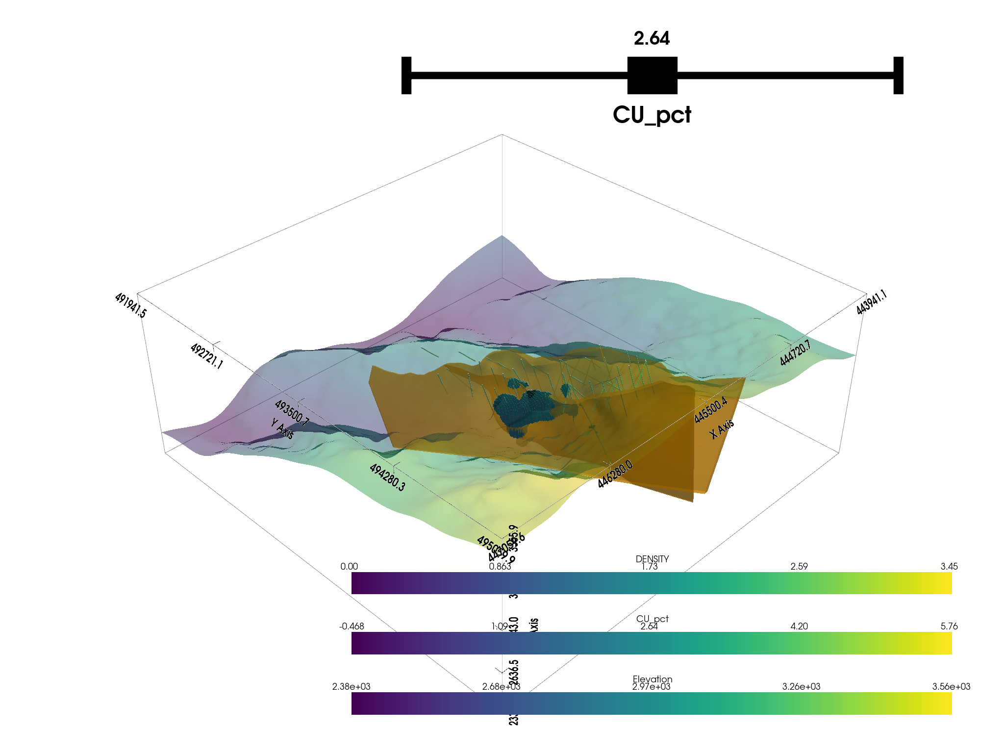
Threshold the volumetric data

thresh_vol = vol.threshold([1.09, 4.20])
print(thresh_vol)

UnstructuredGrid (0x7f90cc7391e0)
  N Cells:    92525
  N Points:   107807
  X Bounds:   4.447e+05, 4.457e+05
  Y Bounds:   4.929e+05, 4.942e+05
  Z Bounds:   2.330e+03, 3.110e+03
  N Arrays:   1

Create a plotting window

p = pv.Plotter()
# Add the bounds axis
p.show_bounds()
p.add_bounding_box()

# Add our datasets
p.add_mesh(topo, opacity=0.5)
p.add_mesh(
    dacite,
    color="orange",
    opacity=0.6,
)
# p.add_mesh(thresh_vol, cmap="coolwarm", clim=vol.get_data_range())
p.add_mesh_threshold(vol, scalars="CU_pct", show_edges=True)


# Add the assay logs: use a tube filter that varius the radius by an attribute
p.add_mesh(assay.tube(radius=3), cmap="viridis")

p.show()

Export the model data

# Create DataFrame
df = pd.DataFrame(vol.cell_centers().points, columns=['x', 'y', 'z'])

# Add the array data to the DataFrame
for name in vol.array_names:
    df[name] = vol.get_array(name)

# set the index to the cell centroids
df.set_index(['x', 'y', 'z'], drop=True, inplace=True)

# Write DataFrame to parquet file
df.to_parquet('block_model_copper.parquet')

Profile

profile = ProfileReport(df.reset_index(), title="Profiling Report")
profile.to_file("block_model_copper_profile.html")

Summarize dataset:   0%|          | 0/5 [00:00<?, ?it/s]
Summarize dataset:   0%|          | 0/9 [00:00<?, ?it/s, Describe variable:y]
Summarize dataset:  11%|█         | 1/9 [00:00<00:02,  3.51it/s, Describe variable:y]
Summarize dataset:  11%|█         | 1/9 [00:00<00:02,  3.51it/s, Describe variable:z]
Summarize dataset:  22%|██▏       | 2/9 [00:00<00:01,  3.51it/s, Describe variable:x]
Summarize dataset:  33%|███▎      | 3/9 [00:02<00:01,  3.51it/s, Describe variable:CU_pct]
Summarize dataset:  44%|████▍     | 4/9 [00:02<00:02,  1.84it/s, Describe variable:CU_pct]
Summarize dataset:  44%|████▍     | 4/9 [00:02<00:02,  1.84it/s, Get variable types]
Summarize dataset:  50%|█████     | 5/10 [00:02<00:02,  1.84it/s, Get dataframe statistics]
Summarize dataset:  55%|█████▍    | 6/11 [00:02<00:02,  1.84it/s, Calculate auto correlation]
Summarize dataset:  64%|██████▎   | 7/11 [00:03<00:02,  1.82it/s, Calculate auto correlation]
Summarize dataset:  64%|██████▎   | 7/11 [00:03<00:02,  1.82it/s, Get scatter matrix]
Summarize dataset:  26%|██▌       | 7/27 [00:03<00:11,  1.82it/s, scatter x, x]
Summarize dataset:  30%|██▉       | 8/27 [00:04<00:09,  2.05it/s, scatter x, x]
Summarize dataset:  30%|██▉       | 8/27 [00:04<00:09,  2.05it/s, scatter y, x]
Summarize dataset:  33%|███▎      | 9/27 [00:04<00:07,  2.29it/s, scatter y, x]
Summarize dataset:  33%|███▎      | 9/27 [00:04<00:07,  2.29it/s, scatter z, x]
Summarize dataset:  37%|███▋      | 10/27 [00:04<00:06,  2.56it/s, scatter z, x]
Summarize dataset:  37%|███▋      | 10/27 [00:04<00:06,  2.56it/s, scatter CU_pct, x]
Summarize dataset:  41%|████      | 11/27 [00:04<00:05,  2.83it/s, scatter CU_pct, x]
Summarize dataset:  41%|████      | 11/27 [00:04<00:05,  2.83it/s, scatter x, y]
Summarize dataset:  44%|████▍     | 12/27 [00:05<00:04,  3.06it/s, scatter x, y]
Summarize dataset:  44%|████▍     | 12/27 [00:05<00:04,  3.06it/s, scatter y, y]
Summarize dataset:  48%|████▊     | 13/27 [00:05<00:04,  3.28it/s, scatter y, y]
Summarize dataset:  48%|████▊     | 13/27 [00:05<00:04,  3.28it/s, scatter z, y]
Summarize dataset:  52%|█████▏    | 14/27 [00:05<00:03,  3.48it/s, scatter z, y]
Summarize dataset:  52%|█████▏    | 14/27 [00:05<00:03,  3.48it/s, scatter CU_pct, y]
Summarize dataset:  56%|█████▌    | 15/27 [00:05<00:03,  3.59it/s, scatter CU_pct, y]
Summarize dataset:  56%|█████▌    | 15/27 [00:05<00:03,  3.59it/s, scatter x, z]
Summarize dataset:  59%|█████▉    | 16/27 [00:06<00:02,  3.75it/s, scatter x, z]
Summarize dataset:  59%|█████▉    | 16/27 [00:06<00:02,  3.75it/s, scatter y, z]
Summarize dataset:  63%|██████▎   | 17/27 [00:06<00:02,  3.79it/s, scatter y, z]
Summarize dataset:  63%|██████▎   | 17/27 [00:06<00:02,  3.79it/s, scatter z, z]
Summarize dataset:  67%|██████▋   | 18/27 [00:06<00:02,  4.03it/s, scatter z, z]
Summarize dataset:  67%|██████▋   | 18/27 [00:06<00:02,  4.03it/s, scatter CU_pct, z]
Summarize dataset:  70%|███████   | 19/27 [00:06<00:01,  4.02it/s, scatter CU_pct, z]
Summarize dataset:  70%|███████   | 19/27 [00:06<00:01,  4.02it/s, scatter x, CU_pct]
Summarize dataset:  74%|███████▍  | 20/27 [00:06<00:01,  4.02it/s, scatter x, CU_pct]
Summarize dataset:  74%|███████▍  | 20/27 [00:06<00:01,  4.02it/s, scatter y, CU_pct]
Summarize dataset:  78%|███████▊  | 21/27 [00:07<00:01,  3.94it/s, scatter y, CU_pct]
Summarize dataset:  78%|███████▊  | 21/27 [00:07<00:01,  3.94it/s, scatter z, CU_pct]
Summarize dataset:  81%|████████▏ | 22/27 [00:07<00:01,  4.01it/s, scatter z, CU_pct]
Summarize dataset:  81%|████████▏ | 22/27 [00:07<00:01,  4.01it/s, scatter CU_pct, CU_pct]
Summarize dataset:  85%|████████▌ | 23/27 [00:07<00:00,  4.10it/s, scatter CU_pct, CU_pct]
Summarize dataset:  79%|███████▉  | 23/29 [00:07<00:01,  4.10it/s, Missing diagram bar]
Summarize dataset:  83%|████████▎ | 24/29 [00:07<00:01,  4.59it/s, Missing diagram bar]
Summarize dataset:  83%|████████▎ | 24/29 [00:07<00:01,  4.59it/s, Missing diagram matrix]
Summarize dataset:  86%|████████▌ | 25/29 [00:08<00:01,  2.57it/s, Missing diagram matrix]
Summarize dataset:  86%|████████▌ | 25/29 [00:08<00:01,  2.57it/s, Take sample]
Summarize dataset:  90%|████████▉ | 26/29 [00:08<00:01,  2.57it/s, Detecting duplicates]
Summarize dataset:  93%|█████████▎| 27/29 [00:09<00:00,  3.42it/s, Detecting duplicates]
Summarize dataset:  93%|█████████▎| 27/29 [00:09<00:00,  3.42it/s, Get alerts]
Summarize dataset:  97%|█████████▋| 28/29 [00:09<00:00,  3.42it/s, Get reproduction details]
Summarize dataset: 100%|██████████| 29/29 [00:09<00:00,  3.42it/s, Completed]
Summarize dataset: 100%|██████████| 29/29 [00:09<00:00,  3.22it/s, Completed]

Generate report structure:   0%|          | 0/1 [00:00<?, ?it/s]
Generate report structure: 100%|██████████| 1/1 [00:01<00:00,  1.66s/it]
Generate report structure: 100%|██████████| 1/1 [00:01<00:00,  1.66s/it]

Render HTML:   0%|          | 0/1 [00:00<?, ?it/s]
Render HTML: 100%|██████████| 1/1 [00:00<00:00,  1.85it/s]
Render HTML: 100%|██████████| 1/1 [00:00<00:00,  1.85it/s]

Export report to file:   0%|          | 0/1 [00:00<?, ?it/s]
Export report to file: 100%|██████████| 1/1 [00:00<00:00, 561.26it/s]

Total running time of the script: (0 minutes 21.482 seconds)

Gallery generated by Sphinx-Gallery