Flowsheet Basics

Related Sample objects can be managed as a network. In the Process Engineering/Metallurgy disciplines the network will often be called a flowsheet.

from copy import deepcopy
from typing import Dict

import pandas as pd
from matplotlib import pyplot as plt

from elphick.geomet.flowsheet import Flowsheet
from elphick.geomet.flowsheet.operation import Operation
from elphick.geomet.flowsheet.stream import Stream
from elphick.geomet.utils.data import sample_data

Create some Sample objects

Create an object, and split it to create two more objects.

df_data: pd.DataFrame = sample_data()
obj_strm: Stream = Stream(df_data, name='Feed')
obj_strm_1, obj_strm_2 = obj_strm.split(0.4, name_1='stream 1', name_2='stream 2')

Placeholder random nodes are created for each Sample object. This is done to capture the relationships implicitly defined by any math operations performed on the objects.

for obj in [obj_strm, obj_strm_1, obj_strm_2]:
    print(obj.name, obj.nodes)

Feed [68, 32]
stream 1 [32, 147354623897227054935805936137080412508]
stream 2 [32, 264799010139310533413209377373268495415]

Create a Flowsheet object

This requires passing an Iterable of Sample objects

fs: Flowsheet = Flowsheet.from_objects([obj_strm, obj_strm_1, obj_strm_2])

Print the node object detail

for node in fs.graph.nodes:
    print(fs.graph.nodes[node]['mc'])

<elphick.geomet.flowsheet.operation.Operation object at 0x7f90dbe9ae30>
<elphick.geomet.flowsheet.operation.Operation object at 0x7f90dbe98640>
<elphick.geomet.flowsheet.operation.Operation object at 0x7f90dbe9ad10>
<elphick.geomet.flowsheet.operation.Operation object at 0x7f90dbe988b0>

Note that the random node placeholder integers have been renumbered for readability.

for obj in [obj_strm, obj_strm_1, obj_strm_2]:
    print(obj.name, obj.nodes)

Feed [0, 1]
stream 1 [1, 2]
stream 2 [1, 3]

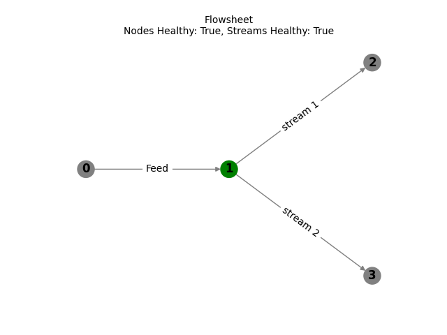
Print the overall network balanced status

NOTE: presently this only includes node balance status edge balance status will assure the mass-moisture balance is satisfied

print(fs.balanced)

True

Plot the network. Imbalanced Nodes will appear red. Later, Imbalanced Edges will also appear red.

fs.plot()
plt

<module 'matplotlib.pyplot' from '/home/runner/work/geometallurgy/geometallurgy/.venv/lib/python3.10/site-packages/matplotlib/pyplot.py'>

Display the weight averages for all edges (streams) in the network (flowsheet)

df_report: pd.DataFrame = fs.report()
df_report

	wet_mass	mass_dry	H2O	Fe	SiO2	Al2O3	LOI
name
Feed	300.0	260.0	13.333333	59.0	3.515385	1.873077	4.0
stream 1	120.0	104.0	13.333333	59.0	3.515385	1.873077	4.0
stream 2	180.0	156.0	13.333333	59.0	3.515385	1.873077	4.0

df_report: pd.DataFrame = fs.report(apply_formats=True)
df_report

	wet_mass	mass_dry	H2O	Fe	SiO2	Al2O3	LOI
name
Feed	300	260	13.3	59.00	3.52	1.87	4.00
stream 1	120	104	13.3	59.00	3.52	1.87	4.00
stream 2	180	156	13.3	59.00	3.52	1.87	4.00

Plot the interactive network using plotly

fig = fs.plot_network()
fig

Plot the Sankey

fig = fs.plot_sankey()
fig

Demonstrate the table-plot

fig = fs.table_plot(plot_type='sankey', table_pos='top', table_area=0.3).update_layout(height=700)
fig

fig = fs.table_plot(plot_type='network', table_pos='bottom', table_area=0.3).update_layout(height=700)
fig

Expand the Network with Math Operators

obj_strm_3, obj_strm_4 = obj_strm_2.split(0.8, name_1='stream 3', name_2='stream 4')
obj_strm_5 = obj_strm_1.add(obj_strm_3, name='stream 5')

fs2: Flowsheet = Flowsheet.from_objects([obj_strm, obj_strm_1, obj_strm_2, obj_strm_3, obj_strm_4, obj_strm_5])

fig = fs2.table_plot(plot_type='sankey', table_pos='left')
fig

Setting Node names

nodes_before: Dict[int, Operation] = fs.nodes_to_dict()
print({n: o.name for n, o in nodes_before.items()})

{0: '0', 1: '1', 2: '2', 3: '3'}

fs.set_node_names(node_names={0: 'node_0', 1: 'node_1', 2: 'node_2', 3: 'node_3'})
nodes_after: Dict[int, Operation] = fs.nodes_to_dict()
print({n: o.name for n, o in nodes_after.items()})

{0: 'node_0', 1: 'node_1', 2: 'node_2', 3: 'node_3'}

Setting Stream data

First we show how to easily access the stream data as a dictionary

stream_data: Dict[str, Stream] = fs.streams_to_dict()
print(stream_data.keys())

dict_keys(['Feed', 'stream 1', 'stream 2'])

We will replace stream 2 with the same data as stream 1.

new_stream: Stream = deepcopy(fs.get_edge_by_name('stream 1'))
# we need to rename to avoid a creating a duplicate stream name
new_stream.name = 'stream 1 copy'
fs.set_stream_data({'stream 2': new_stream})
print(fs.streams_to_dict().keys())

dict_keys(['Feed', 'stream 1', 'stream 1 copy'])

Of course the network is now unbalanced as highlighted in the Sankey

fig = fs.table_plot()
fig

Methods to modify relationships

Sometimes the network that is automatically created may not be what you are after - for example flow may be in the wrong direction. We’ll learn how to modify an existing network, by picking up the network above.

Let’s break the links for the _stream 1_.

fs.reset_stream_nodes(stream="stream 1")
fig = fs.table_plot()
fig

We’ll now break all remaining connections (we could have done this from the start).

fs.reset_stream_nodes()
fig = fs.table_plot()
fig

Now we’ll create some linkages - of course they will be completely rubbish and not balance.

fs.set_stream_parent(stream="stream 1", parent="Feed")
fs.set_stream_child(stream="stream 1", child="stream 1 copy")
fig = fs.table_plot()
fig

Perhaps less useful, but possible, we can build relationships by setting nodes directly.

fs.reset_stream_nodes()
fs.set_nodes(stream="stream 1", nodes=(1, 2))
fs.set_nodes(stream="stream 1 copy", nodes=(2, 3))
fig = fs.table_plot()
fig